2.3 - Horizontal Motion with Stokes Drag

From: Classical Physics / Chapter 2 - Projectile Motion and Air Drag

Introduction

This page derives the time-dependent trajectory of a particle moving through a fluid (such as air or water) in the limit that vicsous forces dominate the motion (see 2.1 Introduction to Air Drag). In this limit, the drag force has a linear velocity dependence and is given by Stokes drag (also called linear drag). It applies to objects with low Reynolds numbers (i.e. small objects or very viscous fluids). The magnitude of the drag force is given by:

F_d = 6\pi \eta r v

and where $r$ is the radius of the sphere and $\eta$ is the dynamic viscosity. In the following derivations, We will simplify this expression for the drag force to the following, where the negative sign indicates that the drag force opposes the motion:

$$F_d = -b v$$

where $b = 6\pi \eta r$ is the drag coefficient.

System Definition: A particle with mass $m$ moves under the influence of linear (Stokes) drag:

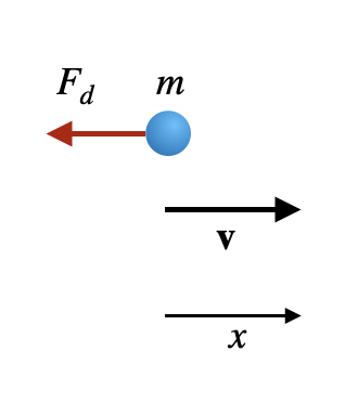
Motion is along the $x$ axis.
Drag force: $F_d = -bv_x$, where $b = 6\pi \eta r$ is the linear drag coefficient.
Initial conditions: $v_{0x}$ and $x_0$. We'll take the starting point as the origin, i.e. $x_0 = 0$.

Goal: Derive the equation of motion for a particle with Stokes drag and solve for $v_x(t)$ and $x(t)$.

The Equation of Motion

According to Newton's second law, the net force on the particle equals its mass times acceleration:

F_{\text{net}} = ma

The only force acting on the particle (assuming no other forces like gravity in the direction of motion) is the drag force $F_d = -bv_x$, where the negative sign indicates it opposes the direction of motion. We also substitute $a = \frac{dv_x}{dt}$:

-bv_x = m\frac{dv_x}{dt}.

Rearranging, we obtain the equation of motion:

Equation of Motion for a Particle with Stokes Drag:

\frac{dv_x}{dt} = -\frac{b}{m}v_x

This is a first-order linear ordinary differential equation. The quantity $b/m$ has units of inverse time and represents the rate at which the x-component of velocity decays.

Analytical Solution for Velocity

To solve the differential equation $\frac{dv_x}{dt} = -\frac{b}{m}v_x$, we can use separation of variables:

\frac{dv_x}{v_x} = -\frac{b}{m}dt

Integrating both sides

\int_{v_{0x}}^{v_x(t)} \frac{dv_x'}{v_x'} = -\frac{b}{m}\int_0^t dt'

gives

\ln\left(\frac{v_x(t)}{v_{0x}}\right) = -\frac{b}{m}t.

Taking the exponential of both sides gives the velocity solution:

Velocity Solution for a Particle with Stokes Drag:

v_x(t) = v_{0x} e^{-\frac{b}{m}t}

This shows that the x-component of velocity decays exponentially with time.

Characteristic Time

The dynamics of this system are characterized by a single time scale, called the characteristic time or relaxation time, defined as:

\tau = \frac{m}{b}

The characteristic time $\tau$ represents the time it takes for the x-component of velocity to decrease by a factor of $e$ (approximately 2.718). It is the natural time scale of the system and determines how quickly the velocity decays.

Using the characteristic time, we can rewrite the equation of motion in a more compact form:

\frac{dv_x}{dt} = -\frac{v_x}{\tau}

Similarly, the velocity solution can be expressed in terms of $\tau$:

Velocity Solution (in terms of $\tau$):

v_x(t) = v_{0x} e^{-t/\tau}

This form makes it clear that the velocity decays exponentially with a time constant $\tau$. At time $t = \tau$, the velocity has decreased to $v_{0x}/e \approx 0.368v_{0x}$.

Analytical Solution for Position

To find the position as a function of time, we integrate the x-component of velocity. Using the velocity solution in terms of $\tau$:

x(t) = \int_0^t v_x(t') dt' = \int_0^t v_{0x} e^{-t'/\tau} dt'

Performing the integration:

x(t) = v_{0x} \int_0^t e^{-t'/\tau} dt' = v_{0x} \left[-\tau e^{-t'/\tau}\right]_0^t

x(t) = v_{0x} \left(-\tau e^{-t/\tau} + \tau\right)

Position Solution (in terms of $\tau$):

x(t) = v_{0x}\tau\left(1 - e^{-t/\tau}\right)

This shows that the position approaches a maximum value of $v_{0x}\tau$ as time goes to infinity. This makes physical sense: as the x-component of velocity decays to zero, the particle stops moving and reaches a final position.

Limiting Behavior of the Position Solution

It's instructive to examine the position solution $x(t) = v_{0x}\tau\left(1 - e^{-t/\tau}\right)$ in two important limits: when time goes to infinity, and when time is much smaller than the characteristic time $\tau$. This both help to understand the behavior of the system and serves as a reality check for the analytical solution.

Limit 1: Long-Time Behavior ($t \to \infty$)

As time approaches infinity, the exponential term $e^{-t/\tau}$ approaches zero. Taking the limit:

\lim_{t \to \infty} x(t) = \lim_{t \to \infty} v_{0x}\tau\left(1 - e^{-t/\tau}\right) = v_{0x}\tau(1 - 0) = v_{0x}\tau

This confirms that the maximum distance the particle can travel is $x_{\max} = v_{0x}\tau$. Physically, this represents the final position where the particle comes to rest (asymptotically) after all its initial kinetic energy has been dissipated by the drag force.

Limit 2: Short-Time Behavior ($t \ll \tau$)

For times much shorter than the characteristic time $\tau$, we can use a Taylor series expansion to approximate the exponential term. The Taylor series for $e^x$ is $e^x \approx 1 + x $. Substituting $x = -t/\tau$ gives $e^{-t/\tau} \approx 1 - \frac{t}{\tau}$. Thus the position solution in the limit $t \ll \tau$ is approximately:

x(t) = v_{0x}\tau\left(1 - e^{-t/\tau}\right) \approx v_{0x}\tau\left(1 - \left(1 - \frac{t}{\tau}\right)\right),

which, after simplifying, gives:

x(t) \approx v_{0x}\tau\left(\frac{t}{\tau}\right) = v_{0x}t.

This result makes physical sense: at very short times (before the drag force has had time to significantly slow the particle), the particle moves approximately with constant velocity $v_{0x}$, so its position increases linearly with time. This is the same behavior we would expect for a particle moving without any drag force.

Key Observations:

The x-component of velocity decays exponentially: $v_x(t) = v_{0x} e^{-t/\tau}$ where $\tau = m/b$
The position approaches a maximum: $x_{\max} = v_{0x}\tau$
The particle never comes to a complete stop in finite time, but approaches zero velocity asymptotically

Example: Motion of a Water Drop in Air

To model the motion of a water drop in air, we can write the characteristic time $\tau$ in terms of the physical units of the problem by substituting $b=6\pi \eta r$ into $\tau = m/b$:

\tau = \frac{m}{6\pi \eta r}.

Let's assume the water drop has a radius $r$ and a density of $\rho_{water} = 1000 \;kg/m^3$. The mass of the water drop is $m = \rho_{water} V = \rho_{water} \frac{4}{3}\pi r^3$. The characteristic time is then:

\tau = \frac{\rho_{water} \frac{4}{3}\pi r^3}{6\pi \eta r} = \frac{2}{9}\frac{\rho_{water} r^2}{\eta}.

In order for Stokes drag to be appropriate, the Reynolds number must be less than 1. We'll use a $r=15 \mu m$ fog droplet, since we found the Reynods number to be 0.01 on the previous page (2.1 Introduction to Air Drag). The dynamic viscosity of air is $\eta = 1.81\times 10^{-5}$ Pa s. The characteristic time is then:

\begin{aligned}\tau & = \frac{2}{9}\frac{\rho_{water} r^2}{\eta} \\ & = \frac{2}{9}\frac{1000 \;kg/m^3 (1.5\times 10^{-5} \;m)^2}{1.81\times 10^{-5} \;Pa \cdot s} \\ & = 0.0028 \;s. \end{aligned}

This shows that a 15 $\mu$m water drop can only move through air for about 3 micro-seconds before it slows down substantially.

We can estimate the maximum distance traveled by the water drop by multiplying the characteristic time by the initial velocity. For a fod droplet, we'll use an initial velocity of $v_{0x} = 0.01 \;m/s$:

x_{\max} = v_{0x} \tau = 0.01 \;m/s \times 0.0028 \;s = 0.000028 \;m = 28 \; \mu m.

This shows that a 15 $\mu$m water drop can only move through air about the distance of its diameter before being slowed by the air's viscosity.

For larger objects or higher speeds, the drag force is often better modeled as quadratic in velocity ($F_d \propto v^2$), which leads to different dynamics.

Viscous Drag Solution

Radius (r): 15 μm

Initial Velocity (v₀ₓ): 0.01 m/s

Time Range (ms): 10.0

Analytical solution for position with Stokes drag

Using the Plot

Position curve: Shows how the particle's position changes over time. Notice how it approaches the maximum value $v_{0x}\tau$ asymptotically.
Adjust parameters: Use the sliders to change the radius, initial x-component of velocity, and time range to see how they affect the solutions.

Parameters

The plot uses the following default parameters for a water drop in air:

Radius: $1 \;\mu \text{m} \leq r \leq 200 \;\mu \text{m} $
Density of water drop: $\rho_{water} = 1000$ kg/m³
Dynamic viscosity of air: $\eta = 1.81 \times 10^{-5}$ Pa·s
Initial x-component of velocity: $0.001 \;m/s \leq r \leq 0.2 m/s $
Mass of drop: $m = \rho_{water} \frac{4}{3}\pi r^3$ (calculated from radius)
Drag coefficient: $b = 6\pi \eta r$ (Stokes drag)
Characteristic time: $\tau = m/b$
Maximum distance: $x_{\max} = v_{0x}\tau$

Summary

Stokes Drag: For low Reynolds numbers (Re < 1), the drag force on a sphere is $F_d = 6\pi \eta r v = -bv$, where $b = 6\pi \eta r$ is the drag coefficient.
Velocity Solution: The velocity decays exponentially: $v_x(t) = v_{0x} e^{-t/\tau}$, where $\tau = m/b$ is the characteristic time.
Position Solution: The position approaches a maximum asymptotically: $x(t) = v_{0x}\tau(1 - e^{-t/\tau})$, with $x_{\max} = v_{0x}\tau$.
Characteristic Time: For a water drop, $\tau = \frac{2}{9}\frac{\rho_{water} r^2}{\eta}$ determines how quickly the drop slows down.
Reynolds Number: Re = $\frac{\rho_{air} v (2r)}{\eta}$ must be less than 1 for Stokes drag to be valid. When Re > 1, the flow regime changes and Stokes drag no longer applies.
Physical Applications: Stokes drag applies to very small objects (like fog droplets) or very viscous fluids, where viscous forces dominate over inertial forces.