2.4 - Vertical Motion with Stokes Drag

From: Classical Physics / Chapter 2 - Projectile Motion and Air Drag

Introduction

This page continues our exploration of objects moving under the influence of Stokes drag that is applicable to motion in viscous fluids or microscopic particles moving slowly through air. This page examines an object falling through a fluid (such as air), under the influence of gravity and Stokes drag.

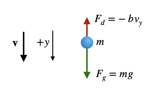
System Definition: A particle with mass $m$ moves under the influence of linear (Stokes) drag and gravity:

Motion is along the vertical $y$ axis. We define the positive direction $+y$ to point downward.
Drag force: $F_d = -bv_y$, where $b = 6\pi \eta r$ is the linear drag coefficient.
Initial conditions: $v_{0y}$ and $y_0$. We'll take the starting point as the origin, i.e. $y_0 = 0$.

Goal: Derive the equation of motion for a particle with Stokes drag and gravity and solve for $v_y(t)$ and $y(t)$.

The Equation of Motion

According to Newton's second law, the net force on the particle equals its mass times acceleration. We have two forces acting:

Gravitational force: $F_g = mg$ (downward, positive direction)
Drag force: $F_d = -bv_y$ (opposes motion, upward when falling)

\begin{aligned} ma &= F_{\text{net}} \\ &= F_g + F_d \\ &= mg - bv_y \end{aligned}

We substitute $a = \frac{dv_y}{dt}$ and rearrange to obtain:

\frac{dv_y}{dt} = g - \frac{b}{m}v_y.

Following the procedure in the previous lecture, we simplify the equation of motion by introducing the characteristic time:

\tau = \frac{m}{b}

Using this characteristic time scale, we can rewrite the equation of motion as:

Equation of Motion for Linear Drag with Gravity:

\frac{dv_y}{dt} = g - \frac{v_y}{\tau}

Notice that each term in the equation has units of velocity per time, so the equation is dimensionally correct.

Terminal Velocity

Even without solving the equation of motion, we can understand something important about the long-term behavior of the falling object. Imagine an object falling from rest. As its velocity increases, the drag force $bv_y$ increases. As the drag force approachs the gravitational force, the acceleration will asymptotically approach zero

F_{\text{net}} = mg - bv_y \approx 0

and we can rearrange the equation as

$$b v_y= mg.$$

We define the terminal velocity as the object's velocity in the limit of infinite time:

Terminal Velocity:

v_{\text{term}} = \frac{mg}{b} = g\tau .

At terminal velocity, the object falls at a constant speed. This represents the long-term behavior: regardless of the initial velocity, the object will eventually approach this terminal velocity. The time scale for reaching terminal velocity is approximately $\tau$.

The terminal velocity depends on:

Mass: Heavier objects have higher terminal velocities (proportional to $m$)
Drag coefficient: Objects with larger drag coefficients have lower terminal velocities (inversely proportional to $b$)
Gravitational acceleration: Higher $g$ leads to higher terminal velocity (proportional to $g$)

This analysis shows that we can understand the asymptotic behavior of the system without needing to solve the full differential equation. The complete solution (derived below) will confirm that the velocity indeed approaches this terminal value exponentially.

Analytical Solution for Velocity

To solve the equation of motion $\frac{dv_y}{dt} = g - \frac{v_y}{\tau}$, we use separation of variables:

\frac{dv_y}{g\tau - v_y} = \frac{dt}{\tau}

Integrating both sides with the initial condition $v_y(0) = v_{0y}$:

\int_{v_{0y}}^{v_y} \frac{dv_y'}{g\tau - v_y'} = \int_0^t \frac{dt'}{\tau}

The left side can be integrated using the substitution $u = g\tau - v_y'$, giving:

-\ln\left|\frac{g\tau - v_y}{g\tau - v_{0y}}\right| = \frac{t}{\tau}

Taking the exponential of both sides and rearranging gives the solution for the velocity $v_y(t)$:

Velocity Solution:

v_y(t) = g\tau + \left(v_{0y} - g\tau\right) e^{-t/\tau}

This shows that the velocity approaches the terminal velocity $v_{\text{term}} = g\tau$ (which we found earlier) exponentially. If the object starts from rest ($v_{0y} = 0$), the solution simplifies to:

Velocity Solution (starting from rest):

v_y(t) = g\tau \left(1 - e^{-t/\tau} \right)

The characteristic time scale $\tau$ is the time it takes for the velocity to approach its terminal value (specifically, the time to reach $1 - 1/e \approx 63\%$ of the terminal velocity when starting from rest).

Analytical Solution for Position

To find the position as a function of time, we integrate the y-component of velocity:

y(t) = \int_0^t v_y(t') dt' = \int_0^t \left[g\tau + \left(v_{0y} - g\tau\right) e^{-t'/\tau}\right] dt'.

Performing the integration:

\begin{aligned} y(t) &= g\tau t + \left(v_{0y} - g\tau\right) \int_0^t e^{-t'/\tau} dt'\\ &= g\tau t + \left(v_{0y} - g\tau\right) \left[-\tau e^{-t'/\tau}\right]_0^t\\ &= g\tau t + \left(v_{0y} - g\tau\right) \left(-\tau e^{-t/\tau} + \tau\right)\\ &= g\tau t - \tau\left(v_{0y} - g\tau\right)\left(e^{-t/\tau} - 1\right) \end{aligned}

Simplify and substitute the terminal velocity $v_{\text{term}} = g\tau$ to get the position solution:

Position Solution:

y(t) = v_{\text{term}} t + \tau\left(v_{0y} - v_{\text{term}}\right)\left(1 - e^{-t/\tau}\right)

If the object starts from rest ($v_{0y} = 0$), this simplifies to:

y(t) = v_{\text{term}} t - v_{\text{term}}\tau\left(1 - e^{-t/\tau}\right)

For large times, the exponential term becomes negligible, and the position approaches $y(t) \approx g\tau t - g\tau^2$, which is the position of an object moving at terminal velocity with a constant offset.

Key Observations:

The velocity approaches terminal velocity exponentially: $v_y(t) \to v_{\text{term}} = g\tau$ as $t \to \infty$
The characteristic time scale is $\tau$
At $t = \tau$, when starting from rest, the velocity reaches approximately $63\%$ of terminal velocity
For large times, the position grows approximately linearly with time: $y(t) \approx v_{\text{term}} t + \text{constant}$

Physical Interpretation

The linear drag model is most appropriate for:

Low Reynolds numbers: When the flow around the object is laminar (smooth)
Small objects: Such as dust particles, small droplets, or particles in viscous fluids
Low speeds: When the drag force is dominated by viscous effects rather than inertial effects

For larger objects or higher speeds, the drag force is often better modeled as quadratic in velocity ($F_d \propto v^2$), which leads to different dynamics and a different expression for terminal velocity.

Mathematical Summary

Complete Solution:

v_y(t) = g\tau + \left(v_{0y} - g\tau\right) e^{-t/\tau}

y(t) = g\tau t + \tau\left(v_{0y} - g\tau\right)\left(1 - e^{-t/\tau}\right)

v_{\text{term}} = g\tau

These analytical solutions are exact and valid for all times $t \geq 0$. They demonstrate the exponential approach to terminal velocity and the resulting position as a function of time.

Falling Motion of Water Drops with Stokes Drag

Radius = 1.0 mm

Initial height H = 5.0 m

X axis upper limit = 5 ms

Free-fall time: -- ms
Stokes drag fall time: -- ms
Terminal velocity: -- m/s
Reynolds number at impact: --

Example: Water Droplet Falling Through Air

Consider a small water droplet falling through air. For very small droplets (diameter on the order of micrometers), the linear drag model (Stokes drag) is appropriate. The drag coefficient for a sphere in a viscous fluid is given by Stokes' law:

b = 6\pi \eta r

where $\eta$ is the dynamic viscosity of air and $r$ is the radius of the droplet.

For a water droplet with diameter $d = 1$ μm ($r = 0.5$ μm = $5 \times 10^{-7}$ m):

Density of water: $\rho_{\text{water}} = 1000$ kg/m³
Volume: $V = \frac{4}{3}\pi r^3 = \frac{4}{3}\pi (5 \times 10^{-7})^3 \approx 5.24 \times 10^{-19}$ m³
Mass: $m = \rho V \approx 5.24 \times 10^{-16}$ kg
Dynamic viscosity of air: $\eta \approx 1.8 \times 10^{-5}$ Pa·s (at room temperature)
Drag coefficient: $b = 6\pi \eta r = 6\pi (1.8 \times 10^{-5})(5 \times 10^{-7}) \approx 1.70 \times 10^{-10}$ N·s/m
Gravitational acceleration: $g = 9.8$ m/s²

Terminal Velocity

First, we calculate the characteristic time scale:

\tau = \frac{m}{b} = \frac{5.24 \times 10^{-16}}{1.70 \times 10^{-10}} \approx 3.08 \times 10^{-6} \text{ s}

The terminal velocity is then:

v_{\text{term}} = g\tau = (9.8)(3.08 \times 10^{-6}) \approx 3.02 \times 10^{-5} \text{ m/s}

The terminal velocity is approximately $0.0302$ mm/s. This is extremely slow!

Time to Fall 1 Meter

To estimate the time it takes for the droplet to fall 1 meter, we can use the position equation. The characteristic time $\tau \approx 3.08 \times 10^{-6}$ s (calculated above) is about 3 microseconds, which is much shorter than the time to fall 1 meter. Therefore, the droplet reaches terminal velocity almost immediately. For large times (much greater than $\tau$), the position is approximately:

y(t) \approx v_{\text{term}} t - g\tau^2

Setting $y = 1$ m and solving for $t$:

1 \approx v_{\text{term}} t - g\tau^2

t \approx \frac{1 + g\tau^2}{v_{\text{term}}}

Calculating the offset term:

g\tau^2 = (9.8)(3.08 \times 10^{-6})^2 \approx 9.3 \times 10^{-12} \text{ m}

This offset is negligible compared to 1 meter, so:

t \approx \frac{1 \text{ m}}{3.02 \times 10^{-5} \text{ m/s}} \approx 33,100 \text{ s}

Converting to more convenient units:

t \approx 33,100 \text{ s} \approx 552 \text{ minutes} \approx \mathbf{9.2 \text{ hours}}

It takes approximately 9.2 hours for a 1-micron diameter water droplet to fall 1 meter through air!

This demonstrates why tiny water droplets can remain suspended in the air for extended periods, forming clouds and fog. The extremely small terminal velocity means that even slight air currents can keep these droplets aloft.