2.5 - Projectile Motion with Stokes Drag

From: Classical Physics / Chapter 2 - Projectile Motion and Air Drag

Introduction

When a particle is launched with an initial velocity at an angle $\theta$ with respect to the horizontal, it follows a curved path through space. In the presence of air resistance, the motion becomes more complex than the simple parabolic trajectory of ideal projectile motion. For linear drag (Stokes drag), where the drag force is proportional to velocity, we can solve the problem by decomposing it into independent horizontal and vertical components.

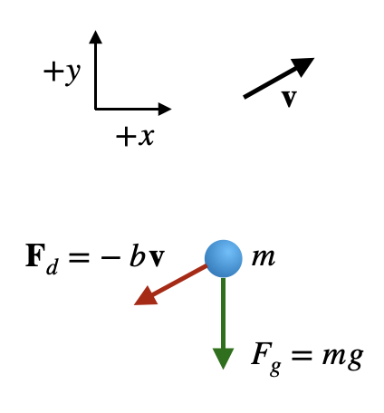
System Definition: A projectile with mass $m$ is launched at an angle $\theta$ with respect to the horizontal and moves under the influence of linear (Stokes) drag and gravity:

We define the positive direction $+y$ to point upward.
Drag force: $F_d = -b(v_x \hat{x} + v_y \hat{y})$, where $b = 6\pi \eta r$ is the linear drag coefficient.
Gravitational acceleration: $g$ (downward, in $-y$ direction)
Initial position: $(x_0, y_0) = (0, 0)$
Initial velocity: $v_{0y}=v_0 \sin\theta$ and $y_0=v_0 \cos\theta$.

Goal: Derive the equation of motion for a particle with Stokes drag and gravity and solve for $v_x(t)$, $v_y(t)$, $x(t)$ and $y(t)$.

Why the Problem Decomposes

The key insight is that the drag force acts independently in each direction:

\begin{aligned} \vec{F}_d &= -b\vec{v}\\ &= -b(v_x \hat{x} + v_y \hat{y})\\ &= -bv_x \hat{x} - bv_y \hat{y}. \end{aligned}

Notice htat the $x$ and $y$ components of the drag force are independent of each other. We will see that this is not true for quadratic, turbulent drag discussed in the next section.

X-component (horizontal):

m\frac{dv_x}{dt} = -bv_x

Y-component (vertical, with $+y$ upward):

m\frac{dv_y}{dt} = -mg - bv_y

Note: On the previous page we defined the positive direction $+y$ to point downward. When analyzing projectile motion, it is more convenient to define the positive direction $+y$ to point upward. With $+y$ pointing upward, the gravitational force is $\vec{F}_g = -mg\hat{y}$.

These equations are uncoupled—the x-component equation doesn't depend on $v_y$ or $y$, and the y-component equation doesn't depend on $v_x$ or $x$. This allows us to solve them independently, using the solutions we derived in previous sections:

The x-component follows the same dynamics as horizontal motion with linear drag (no gravity), which we solved in the linear air drag section.
The y-component follows the same dynamics as vertical motion with linear drag and gravity, which we solved in the vertical air drag section.

Key Insight: Because the drag force is linear and acts independently in each direction, and gravity acts only vertically, the two-dimensional projectile motion problem decomposes into two independent one-dimensional problems. This is a powerful simplification that allows us to use the analytical solutions we've already derived!

Analytical Solutions

Using the characteristic time $\tau = m/b$, we can write the solutions directly from our previous work:

Velocity Solution:

v_x(t) = v_{0x} e^{-t/\tau} = v_0 \cos\theta \cdot e^{-t/\tau}$$ $$v_y(t) = -g\tau + \left(v_0 \sin\theta + g\tau\right) e^{-t/\tau}

Position Solution:

x(t) = v_{0x}\tau\left(1 - e^{-t/\tau}\right) = v_0 \cos\theta \cdot \tau\left(1 - e^{-t/\tau}\right)$$ $$y(t) = -g\tau t + \tau\left(v_0 \sin\theta + g\tau\right)\left(1 - e^{-t/\tau}\right)

Unlike ideal projectile motion (which gives a parabola), this trajectory cannot be written as a simple function $y(x)$. However, we can plot it parametrically by varying $t$ and plotting the resulting $(x, y)$ points.

Skill Check 1: Compare the solutions $v_y(t)$ and $y(t)$ shown above to the corresponding equations derived on the previous page (when the $+y$ direction points downward). Pay particular attention to the signs of the terms. Derive the equations of motion shown above using our assumption that the $+y$ direction points upward. How do the solutions differ?

Physical Interpretation

The trajectory with linear drag differs from ideal projectile motion in several important ways:

Horizontal range is limited: The horizontal velocity decays to zero, so the particle eventually stops moving horizontally. The maximum horizontal distance is $x_{\max} = v_0 \cos\theta \cdot \tau$.
Asymmetric path: The upward and downward portions of the trajectory are not symmetric. The particle falls faster on the way down due to drag opposing the upward motion but aiding the downward motion.
Terminal velocity: On the downward portion, the vertical velocity approaches the terminal velocity $v_{\text{term}} = -g\tau$, meaning the particle falls at a constant speed.
No closed-form $y(x)$: Unlike the parabolic trajectory of ideal projectile motion, we cannot write $y$ as a simple function of $x$; we must use the parametric form.

Interactive Trajectory Plot

Initial Velocity (v₀): 20.0 m/s

Launch Angle (θ): 45°

Drag Coefficient (b): 1.0

Parametric trajectory $(x(t), y(t))$ for projectile motion with linear drag (trajectory stops at ground level, equal x-y scaling)

Maximum horizontal range: calculating... | Terminal velocity: calculating...

Using the Plot

Trajectory curve: The blue curve shows the complete path $(x(t), y(t))$ of the projectile. Notice how it differs from a parabola—the path is asymmetric and the horizontal motion eventually stops. With $+y$ pointing downward, negative $y$ values represent positions above the launch point (ground level).
Initial velocity vector: The red arrow shows the initial velocity vector, with its magnitude and direction determined by $v_0$ and $\theta$. For upward launches ($\theta > 0$), the initial $y$-component of velocity is negative (pointing upward, opposite to the $+y$ direction).
Adjust parameters: Use the sliders to change the initial velocity, launch angle, and drag coefficient to see how they affect the trajectory.
Compare with ideal: Notice how increasing the drag coefficient reduces the range and makes the trajectory more asymmetric.

Parameters

The plot uses the following default parameters:

Mass: $m = 1.0$ (arbitrary units)
Initial velocity: $v_0 = 20.0$ m/s
Launch angle: $\theta = 45°$
Drag coefficient: $b = 1.0$ (arbitrary units)
Gravitational acceleration: $g = 9.8$ m/s²
Characteristic time: $\tau = m/b = 1.0$ s
Terminal velocity: $v_{\text{term}} = g\tau = 9.8$ m/s

Mathematical Summary

Complete Solution (in terms of $\tau = m/b$, with $+y$ downward):

v_x(t) = v_0 \cos\theta \cdot e^{-t/\tau}

v_y(t) = g\tau + \left(-v_0 \sin\theta - g\tau\right) e^{-t/\tau}

x(t) = v_0 \cos\theta \cdot \tau\left(1 - e^{-t/\tau}\right)

y(t) = g\tau t + \tau\left(-v_0 \sin\theta - g\tau\right)\left(1 - e^{-t/\tau}\right)

These analytical solutions are exact and demonstrate how the two-dimensional problem decomposes into independent one-dimensional problems. The horizontal motion is pure exponential decay, while the vertical motion combines gravity with exponential approach to terminal velocity.

Time of Flight

For a projectile launched from ground level ($y_0 = 0$), the time of flight is the time when the particle returns to $y = 0$. This must be found numerically by solving:

g\tau t + \tau\left(-v_0 \sin\theta - g\tau\right)\left(1 - e^{-t/\tau}\right) = 0

For upward launches ($\theta > 0$), we have $v_{0y} = -v_0 \sin\theta < 0$, so the particle starts with negative $y$ (above ground) and negative $v_y$ (moving upward). There are typically two solutions: $t = 0$ (launch) and $t = t_f$ (landing). The landing time $t_f$ can be found numerically. For large drag coefficients or small initial velocities, the particle may not return to ground level if the upward component is too weak.