2.2 - Introduction to Fluid Drag

Sliding Friction: A Review

Before we explore air drag, it's useful to recall the behavior of sliding friction. When an object slides across a solid surface, the frictional force is typically modeled as:

where $\mu_k$ is the coefficient of kinetic friction and $N$ is the normal force. The key characteristic of sliding friction is that it is independent of velocity. Whether an object moves slowly or quickly, the magnitude of the frictional force remains essentially constant (as long as the normal force and contact conditions don't change). The underlying cause of sliding friction is the microscopic irregularities of the surfaces in contact. As the surfaces are pressed together by the normal force, the irregularities come in contact creating a resistive force that opposes the motion.

Why Air Drag is More Complicated

Air drag, or more generally fluid drag, presents a fundamentally different challenge. Unlike sliding friction, drag forces arise from the interaction between a moving object and the fluid (air, water, etc.) through which it moves. This interaction is governed by the principles of fluid dynamics, which are far more complex than the simple contact forces of solid friction.

The figure below shows fluid streamlines around a sphere moving with increasing speed. This visualization illustrates the transition from laminar to turbulent flow as the speed increases. At low speeds, the flow is smooth and orderly (laminar), with streamlines that follow predictable paths around the sphere. As the speed increases, the flow becomes more chaotic, with eddies and vortices forming in the wake behind the sphere, characteristic of turbulent flow. This transition dramatically affects the drag force experienced by the object.

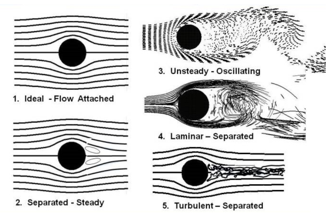
Figure 1: Fluid streamlines around a sphere moving with increasing speed, showing the transition from laminar (smooth, orderly) flow to turbulent (chaotic, with eddies) flow. Source: NASA Glenn Research Center.

Fluid Dynamics and Turbulence

When an object moves through a fluid, many physical processes affect the dynamics of the flow:

• Viscous forces: The fluid has internal friction (viscosity) that resists relative motion between adjacent layers of fluid. This creates a "sticky" effect that opposes the object's motion.
• Pressure forces: The object must push fluid out of its way, creating pressure differences between the front and back of the object. These pressure gradients contribute to the drag force.
• Turbulence: At higher speeds, the flow becomes turbulent rather than smooth (laminar). Turbulent flow involves chaotic, swirling motion of the fluid, which dramatically increases energy dissipation and drag.
• Boundary layer effects: A thin layer of fluid near the object's surface moves with the object (or is slowed by it), creating complex velocity gradients.
• Wake formation: Behind the object, the fluid may separate from the surface, creating vortices and a low-pressure wake region that pulls the object backward.

All of these effects depend on the object's velocity, shape, size, and the properties of the fluid (density, viscosity). This makes drag a much more complicated phenomenon than simple sliding friction and provides job security for countless mechanical engineers.

The Drag Force and Drag Coefficient

In general, the drag force on an object moving through a fluid can be expressed as:

where:

• $F_d$ is the drag force [$N$]
• $C_d$ is the drag coefficient [dimensionless]
• $\rho$ is the fluid density [$kg/m^3$]
• $A$ is the cross-sectional area of the object (projected area perpendicular to the direction of motion) [$m^2$]
• $v$ is the speed of the object relative to the fluid [$m/s$]

The drag coefficient $C_d$ is velocity-dependent, i.e. it is generally not a constant. It depends on many factors including the object's shape, surface roughness, orientation, and most importantly, the Reynolds number, which characterizes the flow regime.

Note that if the drag coefficient were constant, the drag force would be proportional to the square of the velocity $F_d = -cv^2$, where $c=\frac{1}{2} C_d \rho A$. For many of everyday objects moving at moderate speeds through air (i.e. baseballs, cars, skydivers, you walking to class, etc.), this is not a bad approximation. So, it is common to approximate the drag force as having a quadratic dependence on the velocity as a first appeoxomation for most situations.

The Reynolds Number

The Reynolds number is the ratio of inertial forces to viscous forces in the fluid. It is a dimensionless quantity that characterizes the nature of fluid flow around an object. It is defined as:

where:

• $\rho$ is the fluid density [$kg/m^3$]
• $v$ is the characteristic velocity of the object [$m/s$]
• $L$ is a characteristic length (e.g., diameter for a sphere) [$m$]
• $\eta$ is the dynamic viscosity of the fluid [$Pa·s$]

Note: the characteristic length $L$ is easily defined for geometric shapes like spheres, cylinders, plates, etc. It is usually taken to be the diameter of a sphere, the width of a flat plate, etc. The characteristic length of more complex shames is usually estimated as the maximum dimension of the object.

Velocity Dependence in Real Experiments

In real experiments, the relationship between drag force and velocity is complex. The figure below shows experimental data for the drag coefficient of a smooth sphere as a function of the Reynolds number. This graph illustrates how $C_d$ changes dramatically across different flow regimes, from the Stokes regime at low Reynolds numbers to the turbulent regime at high Reynolds numbers.

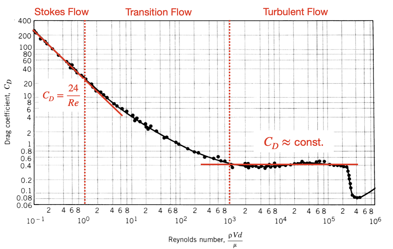
Figure 2: Log-log plot of the drag coefficient as a function of Reynolds number for a smooth sphere as measured from wind tunnel experiments. Source: Munson, et al., 1990, Fundamentals of Fluid Mechanics.

As indicated in Figure 2, the drag force is generally divided into three regimes:

• Re < 1: Laminar/Stokes Flow. In this regime, the flow is dominated by viscous forces. The streamlines are smooth and orderly. The drag coefficient is empirically found to be $C_d = 24/\text{Re}$ and the drag force is thus proportional to the velocity, i.e. $F_d = -bv$. This is the regime for very small objects or very viscous fluids.
• 1 < Re < 1000: Transitional Flow. In this regime, viscous forces and inertial forces are both important. The flow is still smooth, but becomes increasingly irregular. The drag force transitions from having a linear dependence on the velocity to a quadratic dependence. The drag coefficient is empirically found to be $C_d = 10/\text{Re}^{1/2}$ not proportional to the velocity,
• Re > 1000: Turbulent/Quadratic Flow The flow is dominated by inertial forces. The streamlines are chaotic and swirling. In this regime, the drag coefficient is approximatley constant and the drag force is proportional to the square of the velocity, i.e. $F_d = -cv^2$. For very high Reynolds numbers, the drag coefficient exhibits more complex dependence on the Reynolds number, but this behaviour is beyond the scope of this course.

For many practical purposes, we can approximate the drag force using simpler models:

• Linear (Stokes)drag: $F_d = -bv$ (valid at low speeds, small objects, or high viscosity)
• Quadratic (Turbulent) drag: $F_d = -cv^2$ (valid at higher speeds, larger objects, or low viscosity)

These approximations work because, over a limited range of velocities, the drag coefficient $C_d$ is either approximately constant (when the Reynolds number is $Re >3000$ and the flow is turbulent) or varies inversely with respect to velocity (when the Reynolds number is $Re < 1$ and the flow is laminar). The linear approximation is particularly good for very small objects or very viscous fluids (Stokes flow), while the (turbulent) approximation is better for larger objects at moderate to high speeds in air.

Important: The linear and quadratic drag models are approximations that capture the dominant behavior in specific regimes. In reality, the drag coefficient changes with velocity, and the full relationship is more complex.

Stokes Drag

At very low Reynolds numbers, viscous forces dominate. The flow is laminar and smooth. In 1851, George Gabriel Stokes derived the drag force for a sphere as:

where $r$ is the radius of the sphere and $\eta$ is the dynamic viscosity. This is a linear drag law—the force is directly proportional to velocity. Stokes drag applies to:

• Very small objects (e.g., dust particles, pollen)
• Very slow motion
• Very viscous fluids

In this regime, the drag coefficient is inversely proportional to the Reynolds number: $C_d \propto 1/\text{Re}$.

Deriving Stokes Drag from the General Drag Formula

It's instructive to see how Stokes drag emerges from the general quadratic drag formula at low Reynolds numbers. This connection demonstrates how the velocity dependence changes when the drag coefficient itself depends on velocity through the Reynolds number.

We start with the general drag formula:

For a sphere at low Reynolds numbers ($\text{Re} < 1$), the drag coefficient is empirically found to be $C_d = 24/\text{Re}$ (see Figure 2). We substitute in the expression for the Reynolds number $\text{Re} = \rho v L/\eta$ and set the length $L$ to be the diameter $2r$ of the sphere: $$ \begin{aligned} C_d &= \frac{24}{\text{Re}} \\ &= 24\left(\frac{\eta}{2\rho v r}\right)\\ &= \frac{12\eta}{\rho v r} \end{aligned} $$

Plugging this expression for $C_d$ into the general drag formula, we get: